43 adding chart labels in excel
Charts, Graphs & Visualizations by ChartExpo - Google Workspace ChartExpo for Google Sheets has a number of advance charts types that make it easier to find the best chart or graph from charts gallery for marketing reports, agile dashboards, and data analysis: 1. Sankey Diagram 2. Bar Charts 3. Line Graphs (Run Chart) 4. Pie and Donut Charts (Opportunity Charts, Ratio chart) 5. › solutions › excel-chatHow to Insert Axis Labels In An Excel Chart | Excelchat We have a sample chart as shown below; Figure 2 – Adding Excel axis labels. Next, we will click on the chart to turn on the Chart Design tab; We will go to Chart Design and select Add Chart Element; Figure 3 – How to label axes in Excel . In the drop-down menu, we will click on Axis Titles, and subsequently, select Primary Horizontal Figure ...
Box Plots | JMP Visualize and numerically summarize the distribution of continuous variables.
Adding chart labels in excel
How to Use Excel Pivot Table GetPivotData - Contextures Excel Tips At the top left of the Excel window, click the File tab. In the list at the left, click Options (or click More, then click Options) In the Excel Options window, at the left, click the Formulas category. Scroll down to the Working with formulas section. To turn off GetPivotData, remove the check mark for this option: How to Create a Dynamic Chart Range in Excel - Trump Excel This dynamic range is then used as the source data in a chart. As the data changes, the dynamic range updates instantly which leads to an update in the chart. Below is an example of a chart that uses a dynamic chart range. Note that the chart updates with the new data points for May and June as soon as the data in entered. chandoo.org › wp › change-data-labels-in-chartsHow to Change Excel Chart Data Labels to Custom Values? May 05, 2010 · The Chart I have created (type thin line with tick markers) WILL NOT display x axis labels associated with more than 150 rows of data. (Noting 150/4=~ 38 labels initially chart ok, out of 1050/4=~ 263 total months labels in column A.) It does chart all 1050 rows of data values in Y at all times.
Adding chart labels in excel. How to Make a Pie Chart in Excel & Add Rich Data Labels to 08/09/2022 · A pie chart is used to showcase parts of a whole or the proportions of a whole. There should be about five pieces in a pie chart if there are too many slices, then it’s best to use another type of chart or a pie of pie chart in order to showcase the data better. In this article, we are going to see a detailed description of how to make a pie chart in excel. Changelog | MapChart Fixed issue where, when typing numbers (1 to 9) in the legend title or labels, the selected color would change. Version 2.14.12 - 29 June 2022. Fixed issue with the Background color picker not being able to be set to a color with transparency. Version 2.14.11 - 28 June 2022. Fixed issue with the Add Pattern dialog showing the wrong colors ... Prevent Overlapping Data Labels in Excel Charts - Peltier Tech 24/05/2021 · Overlapping data labels becomes more of a problem the more points and labels there are and the longer the labels may be, adding horizontal positions adds complexity, as does the possibility of using different data label positions (judicious use of left/right can unoverlap some labels without fine repositioning). Also, care must be taken to keep labels close enough to … Excel Waterfall Chart: How to Create One That Doesn't Suck - Zebra BI Ideally, you would create a waterfall chart the same way as any other Excel chart: (1) click inside the data table, (2) click in the ribbon on the chart you want to insert. ... in Excel 2016 Microsoft decided to listen to user feedback and introduced 6 highly requested charts in Excel 2016, including a built-in Excel waterfall chart.
Get Digital Help This tutorial shows you how to add a horizontal/vertical line to a chart. Excel allows you to combine two types […] September 23, 2022 . ... Label line chart series. ... The Excel Solver is a free add-in that uses objective cells, constraints based on formulas on a worksheet to perform what-if analysis and other decision problems like ... Customize Excel ribbon with your own tabs, groups or commands In the list of commands on the left, click the command you want to add. Click the Add button. Click OK to save the changes. In the right part of the Customize the Ribbon window, right-click on a target custom group and select Hide Command Labels from the context menu. Click OK to save the changes. Power Apps Excel-Style Editable Table - Part 1 - Matthew Devaney As a final touch we will add a label above the gallery with the column header names. Set the label's Fill property to a color that matches your app's theme and make the FontWeight bold. Our gallery now looks like an Excel spreadsheet. Detecting Edited Rows How to Insert Axis Labels In An Excel Chart | Excelchat We have a sample chart as shown below; Figure 2 – Adding Excel axis labels. Next, we will click on the chart to turn on the Chart Design tab; We will go to Chart Design and select Add Chart Element; Figure 3 – How to label axes in Excel . In the drop-down menu, we will click on Axis Titles, and subsequently, select Primary Horizontal Figure ...
Excel Easy: #1 Excel tutorial on the net 9 Analysis ToolPak: The Analysis ToolPak is an Excel add-in program that provides data analysis tools for financial, statistical and engineering data analysis. VBA . Excel VBA (Visual Basic for Applications) is the name of the programming language of Excel. ... Use a line chart if you have text labels, dates or a few numeric labels on the ... Edit titles or data labels in a chart - support.microsoft.com This displays the Chart Tools, adding the Design, Layout, and Format tabs. On the Layout tab, in the Labels group, click Data Labels , and then click the option that you want. For additional data label options, click More Data Label Options , click Label Options if it's not selected, and then select the options that you want. How to Label a Series of Points on a Plot in MATLAB - Video You can label points on a plot with simple programming to enhance the plot visualization created in MATLAB ®. You can also use numerical or text strings to label your points. Using MATLAB, you can define a string of labels, create a plot and customize it, and program the labels to appear on the plot at their associated point. Feedback. How to Display Percentage in an Excel Graph (3 Methods) Then go to the More Options via the right arrow beside the Data Labels. Select Chart on the Format Data Labels dialog box. Uncheck the Value option. Check the Value From Cells option. Then you have to select cell ranges to extract percentage values. For this purpose, create a column called Percentage using the following formula: =E5/C5
Change the look of chart text and labels in Numbers on Mac ...
MS Excel MCQ Quiz - Objective Question with Answer for MS Excel ... The correct answer is G6.. Key Points. MS Excel is in tabular format consisting of rows and columns.; Row numbers ranges from 1 to 1048576; in total 1048576 rows, and Columns ranges from A to XFD; in total 16384 columns. Row runs horizontally while Column runs vertically. Each row is identified by row number, which runs vertically at the left side of the sheet.
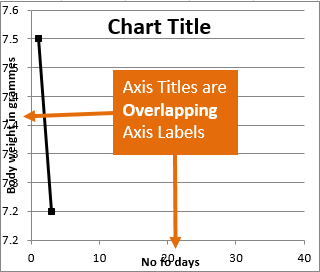
Resize the Plot Area in Excel Chart - Titles and Labels Overlap
How to Create Bins on a Histogram in Tableau - InterWorks The first and second IF conditions check to see if a value is in either set. If it is, then it then creates a label by combining the user input from either parameter with two strings. The first string is just text to make the label easier to read. The second returns the maximum or minimum of the custom bin calculation.

How to add live total labels to graphs and charts in Excel ...
excelchamps.com › blog › speedometerHow to Create a SPEEDOMETER Chart [Gauge] in Excel At this point, you’ll have a chart like below and the next thing is to create the second doughnut chart to add labels. Now, right-click on the chart and then click on “Select Data”. In “Select Data Source” window click on “Add” to enter a new “Legend Entries” and select “Values” column from the second data table.

Add horizontal axis labels - VBA Excel - Stack Overflow
SAS Tutorials: Importing Excel Files into SAS - Kent State University In our case, the dataset we want to import is an Excel file, so select Microsoft Excel Workbook. As you can see, SAS provides you with a large variety of data types to import. Once you've chosen the data source, click Next. Now you need to tell SAS where to find the file you want to import. You can either type the file directory into the text ...

Adding rich data labels to charts in Excel 2013 | Microsoft ...
Free Label Templates for Creating and Designing Labels - OnlineLabels Visit our blank label templates page to search by item number or use the methods below to narrow your scope. Our templates are available in many of the popular file formats so you can create your labels in whatever program you feel most comfortable. You can also narrow your search by selecting the shape of your labels. Search by File Type
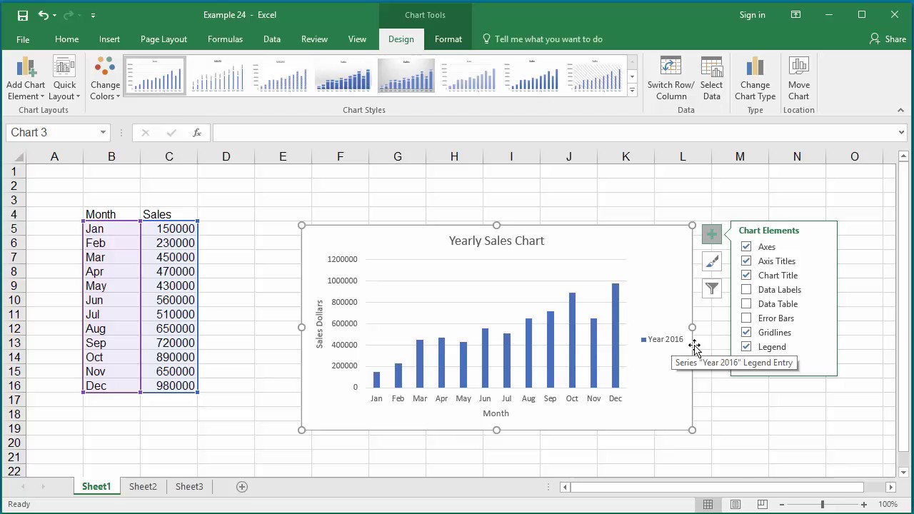
How to Change Elements of a Chart like Title, Axis Titles, Legend etc in Excel 2016
Deployment pipelines, the Power BI Application lifecycle management ... In cases where default labeling is enabled on the tenant, and the default label is valid, if the item being deployed is a dataset or dataflow, the label will be copied from the source item only if the label has protection. If the label is not protected, the default label will be applied to the newly created target dataset or dataflow.
How to add titles to Excel charts in a minute
How to Add Secondary Axis in Excel (3 Useful Methods) - ExcelDemy Firstly, right-click on any of the bars of the chart > go to Format Data Series. Secondly, in the Format Data Series window, select Secondary Axis. Now, click the chart > select the icon of Chart Elements > click the Axes icon > select Secondary Horizontal. We'll see that a secondary X axis is added like this. We'll give the Chart Title as Month.

Add a Data Callout Label to Charts in Excel 2013 – Software ...
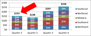
chandoo.org › wp › budget-vs-actual-chart-free-templateFree Budget vs. Actual chart Excel Template - Download May 16, 2018 · Create Budget vs Actual chart with smart labels in Excel – Tutorial. If you are in a hurry to make such a chart, download the template, plug in your values and you are good to go. For instructions on how to create them in Excel, read along. Step 1: Getting the data. Set up your data.

Adding rich data labels to charts in Excel 2013 | Microsoft ...
› bubble-chart-in-excelBubble Chart in Excel - WallStreetMojo A Bubble Chart in Excel is used when we want to represent three sets of data graphically. Out of those three data sets used to make the bubble chart, it shows two-axis of the chart in a series of XY coordinates, and a third set shows the data points. With the help of an Excel Bubble Chart, we can offer the relationship between different datasets.

How to Add Two Data Labels in Excel Chart (with Easy Steps ...
Citing and referencing: Tables and Figures - Monash University Number all Tables and Figures in the order they first appear in the text. Refer to them in the text by their number. For example: As shown in Table 2 ... OR As illustrated in Figure 3 ... Each table or figure should be titled and captioned. For images, photos and paintings see Audio and Visual media in this guide

How to Add Axis Titles in a Microsoft Excel Chart
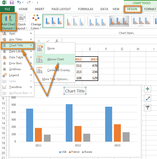
How to add titles to Excel charts in a minute - Ablebits.com In Excel 2013 the CHART TOOLS include 2 tabs: DESIGN and FORMAT . Click on the DESIGN tab. Open the drop-down menu named Add Chart Element in the Chart Layouts group. If you work in Excel 2010, go to the Labels group on the Layout tab. Choose 'Chart Title' and the position where you want your title to display.

How to Add Axis Labels in Excel Charts - Step-by-Step (2022)
r - tmap + labels colors don't match the data - Stack Overflow labels = c ("no drought", "mild drought", "moderate drought", "severe drought", "extreme drought") tm_shape (test) + tm_polygons (col="vcidrought_type", pal =c ("#5dc863ff", "#21908cff", "#3b528bff", "#440154ff", "#000004ff"), labels = labels, title="drought types") + tm_layout (main.title = "vci drought type in sub-saharan africa …

Add Data Labels for Total to Stacked Columns in #Excel | wmfexcel
Charts losing formatting when emailed : r/excel Follow the submission rules -- particularly 1 and 2. To fix the body, click edit. To fix your title, delete and re-post. Include your Excel version and all other relevant information Failing to follow these steps may result in your post being removed without warning. I am a bot, and this action was performed automatically.

How to add live total labels to graphs and charts in Excel ...
How to Build a KPI Dashboard in Excel? [Here is the Easiest Way in 2022] For this, simply select the cells you want to add in the graph and click on Insert to present your data via charts and diagrams. Excel gives you multiple chart choices to select from; bar graphs, pie charts, line graphs, and other visualizations. While assigning charts for your data, keep these things in mind:
How to Add Totals to Stacked Charts for Readability - Excel ...
Excel: How To Convert Data Into A Chart/Graph - Digital Scholarship ... 7: To add axis titles, data labels, legend, trendline, and more, click the graph you just created. A new tab titled "Chart design" should appear. In the upper menu of that tab, you should see a section called "add chart element." 8: In "add chart element," you can customize your graph to your liking . STEP 9: Don't forget to save your work!

How to add or move data labels in Excel chart?
› comparison-chart-in-excelComparison Chart in Excel | Adding Multiple Series Under ... This window helps you modify the chart as it allows you to add the series (Y-Values) as well as Category labels (X-Axis) to configure the chart as per your need. Under Legend Entries ( S eries) inside the Select Data Source window, you need to select the sales values for the years 2018 and year 2019.

How to Change Axis Labels in Excel - TechObservatory
› vba › chart-alignment-add-inMove and Align Chart Titles, Labels, Legends ... - Excel Campus Jan 29, 2014 · *Note: Starting in Excel 2013 the chart objects (titles, labels, legends, etc.) are referred to as chart elements, so I will refer to them as elements throughout this article. The Solution The Chart Alignment Add-in is a free tool ( download below ) that allows you to align the chart elements using the arrow keys on the keyboard or alignment ...

How to Insert Axis Labels In An Excel Chart | Excelchat
Computer Applications Training - University of Arkansas Using Mail Merge, you can generate hundreds of letters, envelopes, labels, or e-mails without having to check each one. Microsoft Word is broken up into Basic, Advanced, and Expert courses. Microsoft Excel. In these classes, participants will learn Excel terminology and how to navigate a workbook, the different ways to enter data, how to format ...

424 How to add data label to line chart in Excel 2016
Build a bar chart visual in Power BI - Power BI | Microsoft Learn Open PowerShell and navigate to the folder you want to create your project in. Enter the following command: PowerShell Copy pbiviz new BarChart You should now have a folder called BarChart containing the visual's files.

How to add data labels from different column in an Excel chart?
What are the Chart elements in Excel | Easy Learn Methods If you need to add or remove elements to the chart, click the plus ( +) button in the upper right corner of the selected chart (2013 and later versions of Excel). Check to add which you want or uncheck which you want to remove. Or you can also remove chart elements in Excel by simply selecting and deleting them. chart elements excel chart elements

Enable or Disable Excel Data Labels at the click of a button ...
Create a bar chart in Excel with start time and duration Steps to create a bar chart in Excel with start time and duration 1 - Arrange the data in Excel 2 - Create a stacked bar chart 3 - Create multiple timeline bar chart 4 - Make the series invisible in chart 5 - Format axis in the chart 6 - Change chart title in Excel Conclusion Steps to create a bar chart in Excel with start time and duration

how to add data labels into Excel graphs — storytelling with data
excel - Macro that selects a product from a slicer so pivot charts ... Any help on this much appreciated. I'm trying to set up a list of product buttons and attach a macro to each one that select the product from the slicer and applies the appropriate axes values but the code below won't work.

Custom data labels in a chart
chandoo.org › wp › change-data-labels-in-chartsHow to Change Excel Chart Data Labels to Custom Values? May 05, 2010 · The Chart I have created (type thin line with tick markers) WILL NOT display x axis labels associated with more than 150 rows of data. (Noting 150/4=~ 38 labels initially chart ok, out of 1050/4=~ 263 total months labels in column A.) It does chart all 1050 rows of data values in Y at all times.

Add or remove data labels in a chart
How to Create a Dynamic Chart Range in Excel - Trump Excel This dynamic range is then used as the source data in a chart. As the data changes, the dynamic range updates instantly which leads to an update in the chart. Below is an example of a chart that uses a dynamic chart range. Note that the chart updates with the new data points for May and June as soon as the data in entered.

Change the format of data labels in a chart
How to Use Excel Pivot Table GetPivotData - Contextures Excel Tips At the top left of the Excel window, click the File tab. In the list at the left, click Options (or click More, then click Options) In the Excel Options window, at the left, click the Formulas category. Scroll down to the Working with formulas section. To turn off GetPivotData, remove the check mark for this option:

How to Add Data Labels to your Excel Chart in Excel 2013
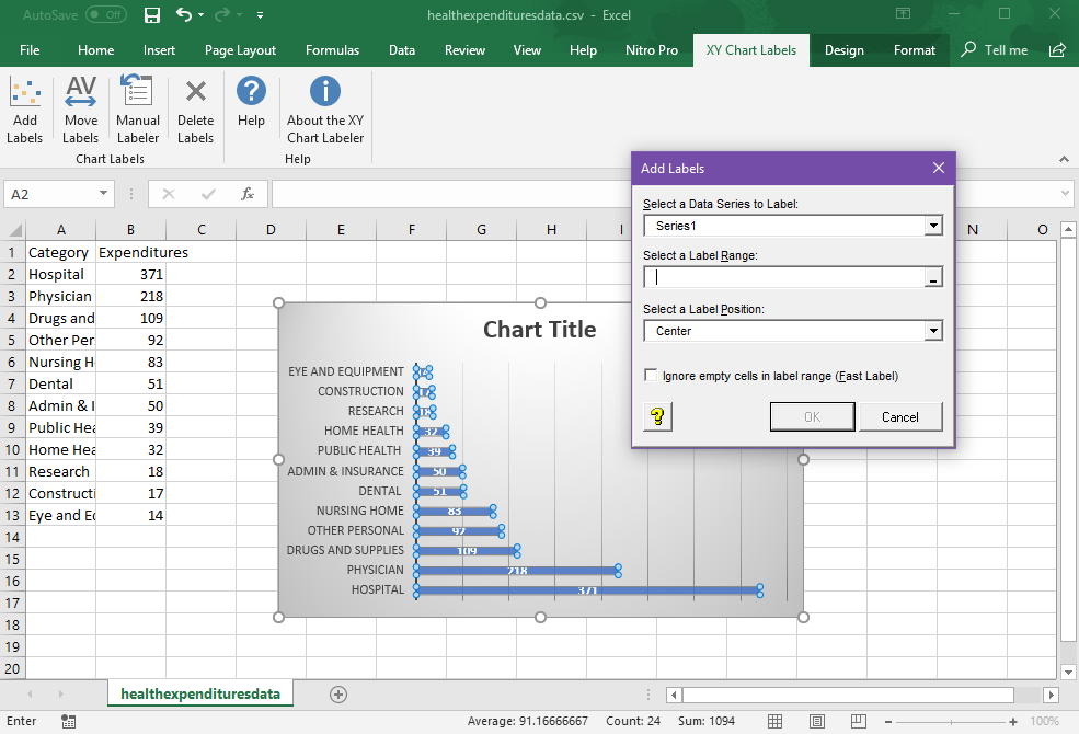
Add Labels to XY Chart Data Points in Excel with XY Chart Labeler

Add data labels and callouts to charts in Excel 365 ...

Excel Charts: Dynamic Label positioning of line series

microsoft excel - Adding data label only to the last value ...

Other Options for Chart Data Labels in PowerPoint 2011 for Mac
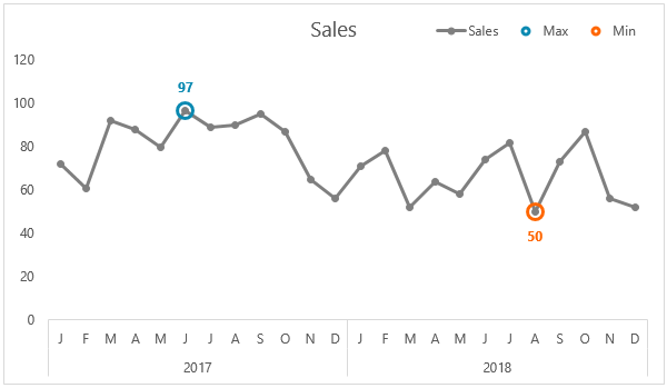
Label Excel Chart Min and Max • My Online Training Hub

How-to Use Data Labels from a Range in an Excel Chart - Excel ...

Is there a way to add data labels as percentages on the ...

Apply Custom Data Labels to Charted Points - Peltier Tech

Add label to Excel chart line • AuditExcel.co.za MS Excel ...

How to Add and Remove Chart Elements in Excel
/simplexct/BlogPic-h7046.jpg)
How to Create a Bar Chart With Labels Above Bars in Excel

how to add data labels into Excel graphs — storytelling with data

How to add data labels from different column in an Excel chart?

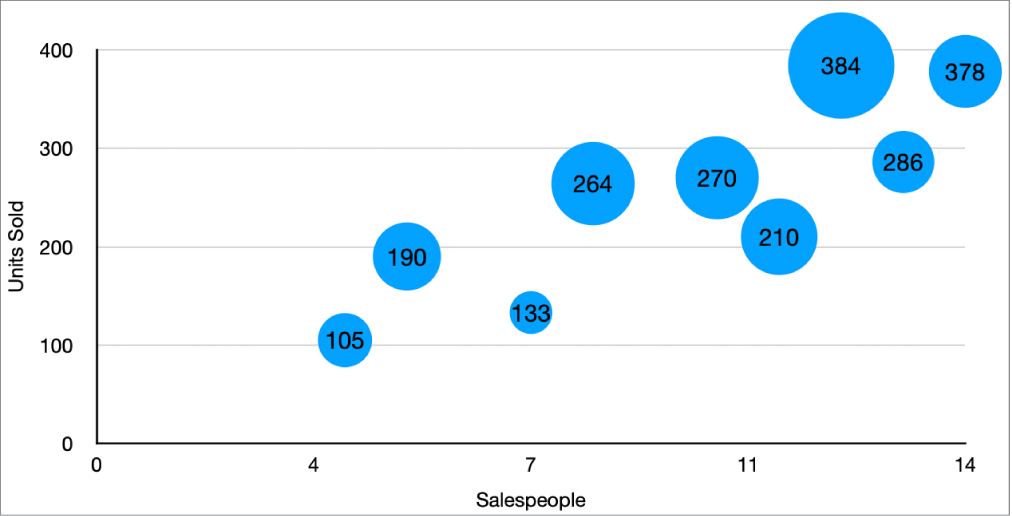
Add data labels to your Excel bubble charts | TechRepublic

Custom data labels in a chart

Adding rich data labels to charts in Excel 2013 | Microsoft ...
Post a Comment for "43 adding chart labels in excel"