41 pivot table excel row labels side by side
multiple fields as row labels on the same level in pivot table Excel ... multiple fields as row labels on the same level in pivot table Excel 2016 I am using Excel 2016. I have data that lists product models along with relevant data and also production volumes by month. Part of the relevant data are about 5 common part columns with the part # that applies to each model under the appropriate column. How to make row labels on same line in pivot table in excel #ExcelMaster, #PivotTable, #ExcelHow to make row labels on same line in pivot table in excelHow to show multiple rows in pivot table in excel
How to Customize Your Excel Pivot Chart Data Labels - dummies The Data Labels command on the Design tab's Add Chart Element menu in Excel allows you to label data markers with values from your pivot table. When you click the command button, Excel displays a menu with commands corresponding to locations for the data labels: None, Center, Left, Right, Above, and Below. None signifies that no data labels ...
Pivot table excel row labels side by side
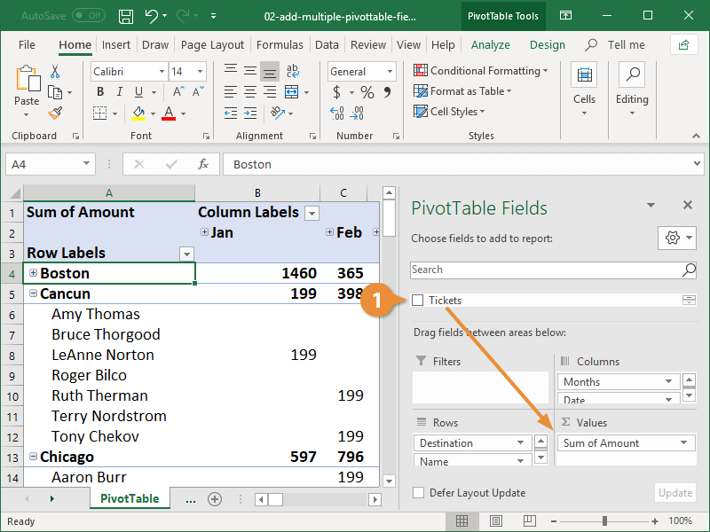
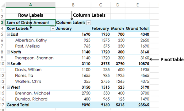
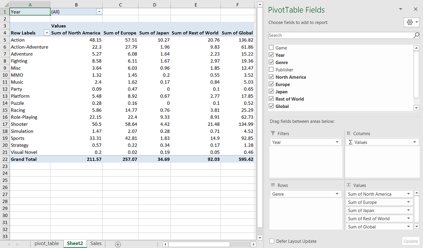
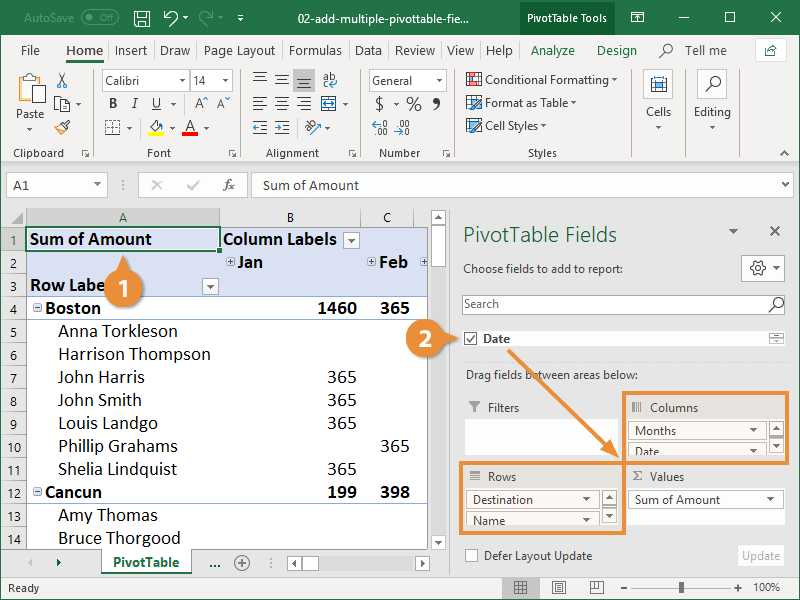
Multi-level Pivot Table in Excel (In Easy Steps) - Excel Easy First, insert a pivot table. Next, drag the following fields to the different areas. 1. Country field to the Rows area. 2. Amount field to the Values area (2x). Note: if you drag the Amount field to the Values area for the second time, Excel also populates the Columns area. Pivot table: 3. Next, click any cell inside the Sum of Amount2 column. 4. Excel 2007 Pivot Table side by side row labels [SOLVED] Excel 2007 Pivot Table side by side row labels Hi Masters In Excel 2003 I could add 2 data elements to the Row label area of the Pivot table. Both items would show up on each row in a different column, this does not happen in 2007 as all items in the row label show up in the same column. How can I revert to the way it was in 2003? Many thanks How To Compare Multiple Lists of Names with a Pivot Table The following are the steps for combining the lists. Make a copy of the '2012' sheet and rename it to 'Combined Data'. In cell E1 add the text "Year". This new column will represent the year for each list of data. Enter "2012" in cell B2 and copy it down to the end of the list. Copy the 2013 data to the bottom of the list on the ...
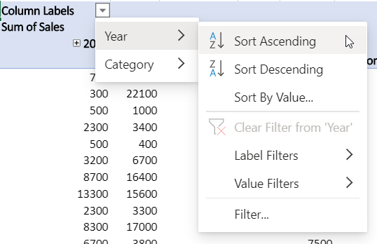
Pivot table excel row labels side by side. The operations currently available are: - Aggregation: consolidate data ... Levels in the pivot table will be stored in MultiIndex objects (hierarchical indexes) on the index and columns of the result DataFrame. Parameters:.. You can display additional column values from the pivot table using pivot->column_name after getting the data from the table using the with method. To avoid errors you have to first define the ... Excel Pivot Table with nested rows | Basic Excel Tutorial Steps 1. Insert your pivot table. Click Insert Menu, under Tables group choose PivotTable. 2. Once you create your pivot table, add all the fields you need to analyze data. How to add the fields Select the checkbox on each field name you desire in the field section. The selected fields are added to the Row Labels area in the layout section. Automatic Row And Column Pivot Table Labels - How To Excel At Excel Select the data set you want to use for your table The first thing to do is put your cursor somewhere in your data list Select the Insert Tab Hit Pivot Table icon Next select Pivot Table option Select a table or range option Select to put your Table on a New Worksheet or on the current one, for this tutorial select the first option Click Ok Excel: How to Sort Pivot Table by Date - Statology Since Excel recognizes the date format, it automatically sorts the pivot table by date from oldest to newest date. However, if we'd like to sort from newest to oldest then we can click on the dropdown arrow next to Row Labels and click Sort Newest to Oldest: The rows in the pivot table will automatically be sorted from newest to oldest: To ...
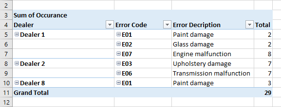
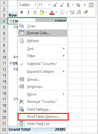
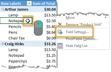
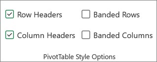
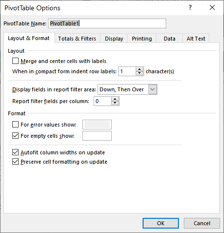
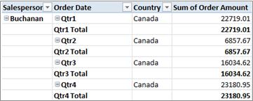
How to add side by side rows in excel pivot table - AnswerTabs To display more pivot table rows side by side, you need to turn on the Classic PivotTable layout and modify Field settings. For example will be used the following table: You have to right-click on pivot table and choose the PivotTable options. Then swich to Display tab and turn on Classic PivotTable layout: Repeat item labels in a PivotTable - support.microsoft.com Right-click the row or column label you want to repeat, and click Field Settings. Click the Layout & Print tab, and check the Repeat item labels box. Make sure Show item labels in tabular form is selected. Notes: When you edit any of the repeated labels, the changes you make are applied to all other cells with the same label. How to Use Excel Pivot Table Label Filters - Contextures Excel Tips To change the Pivot Table option, and allow multiple filters, follow these steps: Right-click a cell in the pivot table, and click PivotTable Options. In the PivotTable Options dialog box, click the Totals & Filters tab. In the Filters section, add a check mark to 'Allow multiple filters per field.'. Click the OK button, to apply the setting ... Pivot Table Row Labels In the Same Line - Beat Excel! First make a pivot table with required fields. Arrange the fields as shown in left picture. Your initial table will look like right picture. Now click on "Error Code" and access field settings. First check "None" option in "Subtotals & Filters" tab to disable totals after every row.
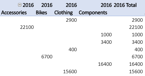
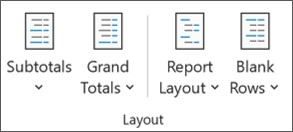
PDF Excel Troubleshooting Row Labels in Pivot Tables In Excel 2007 and earlier, you had to follow these steps: 1. Select the entire pivot table. 2. Copy the pivot table to the clipboard. 3. Use the Paste Special dialog to paste just the Values. This will change the report from a live pivot table to a static report. 4. Select the first blank column cell to the last blank column cell. 5. Pivot Table column label from horizontal to vertical Pivot Table column label from horizontal to vertical. After pivot table and with grouping, some column labels have been showed but the caption is on the top. What i want is put the column header at the left of the row as vertical red text show as below. However, i cannot do this, it said "We cant change this part of pivot table". How to Add Rows to a Pivot Table: 9 Steps (with Pictures) - wikiHow 2. Click anywhere in your pivot table. This opens the pivot table editor on the right side of Google Sheets. 3. Click Add under "Rows." It's in the left side of the pivot table editor. A list of fields will expand on the menu. 4. Click the name of the field you want to add as a row. Design the layout and format of a PivotTable To change the layout of a PivotTable, you can change the PivotTable form and the way that fields, columns, rows, subtotals, empty cells and lines are displayed. To change the format of the PivotTable, you can apply a predefined style, banded rows, and conditional formatting. Windows Web Mac Changing the layout form of a PivotTable
Add Multiple Columns to a Pivot Table | CustomGuide
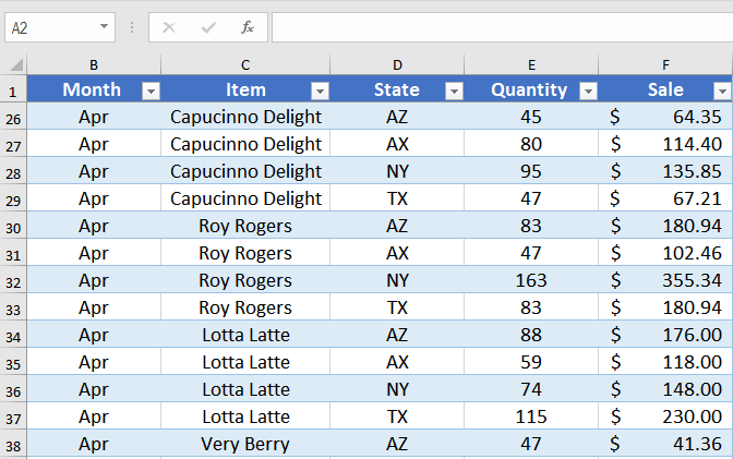
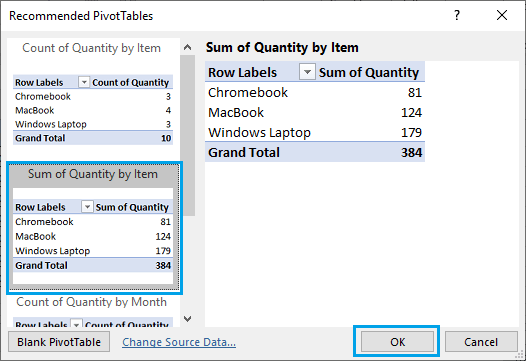
Pivot table row labels side by side - Excel Tutorials - OfficeTuts Excel You can copy the following table and paste it into your worksheet as Match Destination Formatting. Now, let's create a pivot table ( Insert >> Tables >> Pivot Table) and check all the values in Pivot Table Fields. Fields should look like this. Right-click inside a pivot table and choose PivotTable Options…. Check data as shown on the image below.
Pivot table row labels side by side – Excel Tutorials
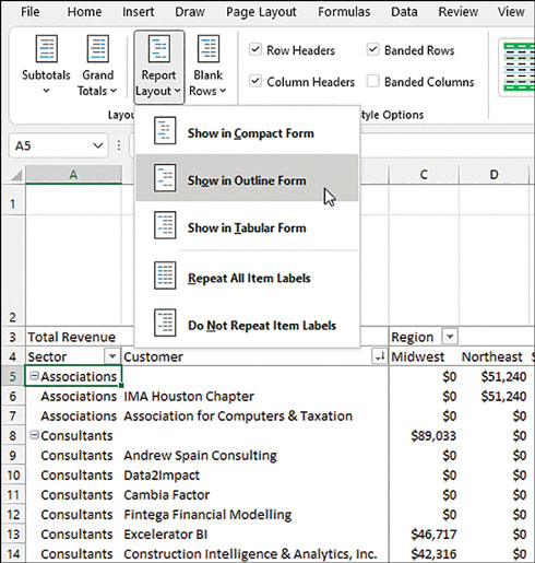
Excel Pivot tables 2007 Row labels side by side - MrExcel Message Board Try selecting a cell in the pivot table and then: PivotTable Tools tab Design tab Report Layout button in the Layout group Select "Show in tabular form" Click to expand... Thank you! This was such an easy solution to a really hard to find problem. You must log in or register to reply here. Similar threads S
Design the layout and format of a PivotTable
Pivot Table row labels in separate columns - YouTube 00:00 Pivot table has multiple fields in one column00:15 Change the Pivot Table field to appear in their own columns00:30 Each column is one Pivot Table fiel...

Excel Pivot Table: How To Show Labels Side by Side - YouTube
Table Headings as Row Headings for Pivot Tables There is a little technic to solve this confusing situation: 1.Insert a new column on the left side of the pivot table. And type in the four elements. 2.Insert a Data filter on this new column, filter the data you want to see and insert slicer. * Beware of scammers posting fake support numbers here.
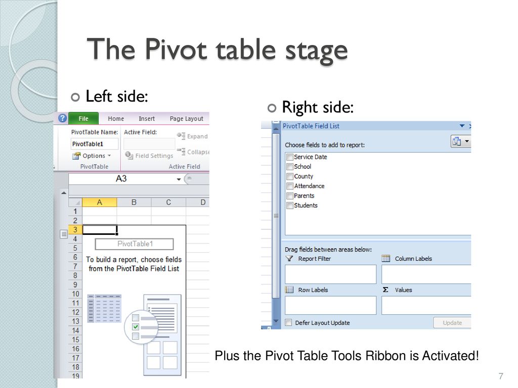
Excel 2016 Pivot Tables Lab Webinar - ppt download
07 Pivot Table side by side row labels - Google Groups - Go to PivotTable Tools, then Options - in the Active Field, select Field Settings - In the Field Settings box, select the 2nd tab 'Layout & Print' - Under 'Show item labels in outline form',...
Instructions for Sorting a Pivot Table by Two Columns | Excelchat
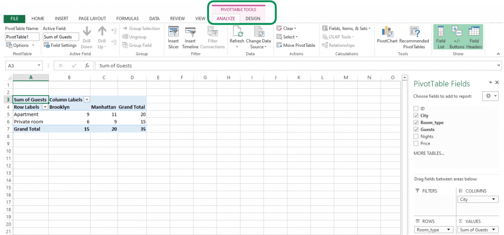
Pivot table row labels in separate columns • AuditExcel.co.za Our preference is rather that the pivot tables are shown in tabular form (all columns separated and next to each other). You can do this by changing the report format. So when you click in the Pivot Table and click on the DESIGN tab one of the options is the Report Layout. Click on this and change it to Tabular form.

Excel Pivot Tables: A Comprehensive Guide
How to make row labels on same line in pivot table? - ExtendOffice Make row labels on same line with PivotTable Options You can also go to the PivotTable Options dialog box to set an option to finish this operation. 1. Click any one cell in the pivot table, and right click to choose PivotTable Options, see screenshot: 2.
How to make row labels on same line in pivot table?
Multi-row and Multi-column Pivot Table - Excel Start Click OK Once the pivot table sheet is created, just like in the previous example, drag the Category and the Product to the Rows section and the Sales Value to the Values section to get the same Multi-Row pivot table we did in the previous example. Next we want to add a column. We will add the Date to the Column section by dragging the field.

Pivot Tables in Excel
How To Compare Multiple Lists of Names with a Pivot Table The following are the steps for combining the lists. Make a copy of the '2012' sheet and rename it to 'Combined Data'. In cell E1 add the text "Year". This new column will represent the year for each list of data. Enter "2012" in cell B2 and copy it down to the end of the list. Copy the 2013 data to the bottom of the list on the ...
How to Save Time and Energy by Analyzing Your Data with Pivot ...
Excel 2007 Pivot Table side by side row labels [SOLVED] Excel 2007 Pivot Table side by side row labels Hi Masters In Excel 2003 I could add 2 data elements to the Row label area of the Pivot table. Both items would show up on each row in a different column, this does not happen in 2007 as all items in the row label show up in the same column. How can I revert to the way it was in 2003? Many thanks

Problems with multiple text fields in a Pivot Table ...
Multi-level Pivot Table in Excel (In Easy Steps) - Excel Easy First, insert a pivot table. Next, drag the following fields to the different areas. 1. Country field to the Rows area. 2. Amount field to the Values area (2x). Note: if you drag the Amount field to the Values area for the second time, Excel also populates the Columns area. Pivot table: 3. Next, click any cell inside the Sum of Amount2 column. 4.

How to make row labels on same line in pivot table?
Design the layout and format of a PivotTable
101 Advanced Pivot Table Tips And Tricks You Need To Know ...
Design the layout and format of a PivotTable

Repeat item labels in a PivotTable
Setting Stable Column Widths in a PivotTable (Microsoft Excel)
Excel Pivot Tables - Filtering Data

Creating Pivot Tables in Excel for Exported Data – Teaching ...
Design the layout and format of a PivotTable

Pivot table row labels in separate columns • AuditExcel.co.za
Automate Pivot Table with Python (Create, Filter and Extract ...
Design the layout and format of a PivotTable
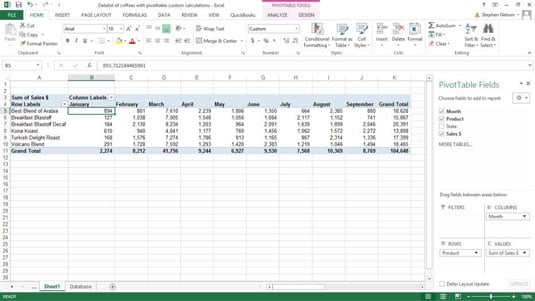
How to Create Custom Calculations for an Excel Pivot Table ...
How to Create Two Pivot Tables in Single Worksheet
The Pivot table tools ribbon in Excel
Customizing a pivot table | Microsoft Press Store
Design the layout and format of a PivotTable

How to make row labels on same line in pivot table?

Pivot Table Row Labels In the Same Line - Beat Excel!
Pivot Table Row Labels In the Same Line - Beat Excel!
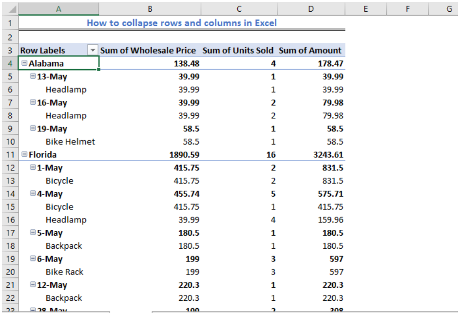
How To Collapse Rows And Columns In Excel - Excelchat | Excelchat

How to show details in pivot table in Excel

Pivot table row labels side by side – Excel Tutorials
Design the layout and format of a PivotTable

Trick to Show Excel Pivot Table Grand Total at Top
Add Multiple Columns to a Pivot Table | CustomGuide

Pivot table row labels in separate columns • AuditExcel.co.za

Excel Pivot Table: How To Show Labels Side by Side - YouTube
MS Excel 2011 for Mac: Display the fields in the Values ...

Excel Pivot Table: How To Show Labels Side by Side - YouTube
Post a Comment for "41 pivot table excel row labels side by side"