45 excel scatter chart data labels
Excel: How to Create a Bubble Chart with Labels - Statology Step 3: Add Labels. To add labels to the bubble chart, click anywhere on the chart and then click the green plus "+" sign in the top right corner. Then click the arrow next to Data Labels and then click More Options in the dropdown menu: In the panel that appears on the right side of the screen, check the box next to Value From Cells within ... Scatter Graph - Overlapping Data Labels - Excel Help Forum The use of unrepresentative data is very frustrating and can lead to long delays in reaching a solution. 2. Make sure that your desired solution is also shown (mock up the results manually). 3. Make sure that all confidential data is removed or replaced with dummy data first (e.g. names, addresses, E-mails, etc.). 4.
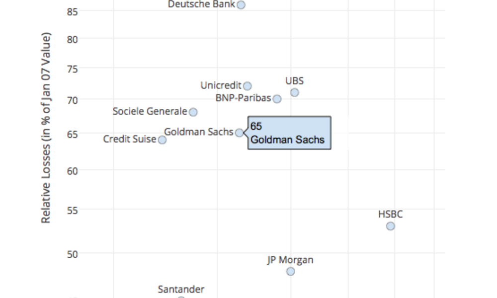
Find, label and highlight a certain data point in Excel scatter graph Add the data point label To let your users know which exactly data point is highlighted in your scatter chart, you can add a label to it. Here's how: Click on the highlighted data point to select it. Click the Chart Elements button. Select the Data Labels box and choose where to position the label.

Excel scatter chart data labels
Improve your X Y Scatter Chart with custom data labels - Get Digital Help Select the x y scatter chart. Press Alt+F8 to view a list of macros available. Select "AddDataLabels". Press with left mouse button on "Run" button. Select the custom data labels you want to assign to your chart. Make sure you select as many cells as there are data points in your chart. Press with left mouse button on OK button. Back to top Add or remove data labels in a chart - support.microsoft.com Click the data series or chart. To label one data point, after clicking the series, click that data point. In the upper right corner, next to the chart, click Add Chart Element > Data Labels. To change the location, click the arrow, and choose an option. If you want to show your data label inside a text bubble shape, click Data Callout. Excel 2016 for Windows - Missing data label options for scatter chart ... Replied on October 12, 2017. You need to use the Add Chart Element tool: either use the + at top right corner of chart, or use Chart Tools (this tab shows up only when a chart is selected) | Design | Add Chart Element. By default this will display the y-values but the Format Labels dialog lets you pick a range. best wishes.
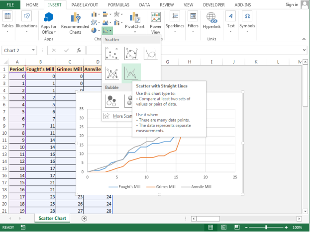
Excel scatter chart data labels. excel - How to label scatterplot points by name? - Stack Overflow This is what you want to do in a scatter plot: right click on your data point. select "Format Data Labels" (note you may have to add data labels first) put a check mark in "Values from Cells". click on "select range" and select your range of labels you want on the points. Scatter chart horizontal axis labels | MrExcel Message Board Apr 26, 2011. #3. Use a Line chart (rather than a XY Scatter chart) and you can have any text in the X values. If you must use a XY Chart, you will have to simulate the effect. Add a dummy series which will have all y values as zero. Then, add data labels for this new series with the desired labels. Locate the data labels below the data points ... buow.nlp-ostsee.de Solution: X-axis or horizontal axis: Number of games. Y-axis or vertical axis: Scores. Now, the scatter graph will be: Note: We can also combine scatter plots in multiple plots per sheet to read and understand the higher-level formation in data sets containing multivariable, notably more than two variables. Scatter > plot Matrix. Excel 2007 : Labels for Data Points on a Scatter Chart Re: Labels for Data Points on a Scatter Chart The addin is not required by anybody receiving your workbook. The addin will link the data label to a cell. If the cell changes the data label will change. New data points will not automatically be linked to new cells. That would require the use of the addin, in order to avoid do it manually.
Excel Chart Vertical Axis Text Labels • My Online Training Hub 14.04.2015 · So all we need to do is get that bar chart into our line chart, align the labels to the line chart and then hide the bars. We’ll do this with a dummy series: Copy cells G4:H10 (note row 5 is intentionally blank) > CTRL+C to copy the cells > select the chart > CTRL+V to paste the dummy data into the chart. How to display text labels in the X-axis of scatter chart in Excel? Display text labels in X-axis of scatter chart. Actually, there is no way that can display text labels in the X-axis of scatter chart in Excel, but we can create a line chart and make it look like a scatter chart. 1. Select the data you use, and click Insert > Insert Line & Area Chart > Line with Markers to select a line chart. See screenshot: How to Make a Scatter Plot in Excel and Present Your Data - MUO Add Labels to Scatter Plot Excel Data Points. You can label the data points in the X and Y chart in Microsoft Excel by following these steps: Click on any blank space of the chart and then select the Chart Elements (looks like a plus icon). Then select the Data Labels and click on the black arrow to open More Options. Analytic Quick Tips - Building Data Labels Into an Excel Scatter Chart ... August 2014 - Building Data Labels Into an Excel Scatter Chart - Made Easy Adding data labels to Excel scatter charts is notoriously difficult as there is no built-in ability in Excel to add data labels. While Microsoft does have a knowledge base page to add data labels, it is difficult to follow.
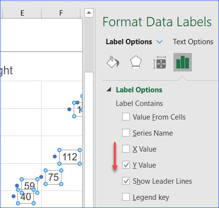
How to use a macro to add labels to data points in an xy scatter chart ... In Microsoft Excel, there is no built-in command that automatically attaches text labels to data points in an xy (scatter) or Bubble chart. However, you can create a Microsoft Visual Basic for Applications macro that does this. This article contains a sample macro that performs this task on an XY Scatter chart. However, the same code can be used for a Bubble Chart. How to Add Labels to Scatterplot Points in Excel - Statology Step 3: Add Labels to Points. Next, click anywhere on the chart until a green plus (+) sign appears in the top right corner. Then click Data Labels, then click More Options…. In the Format Data Labels window that appears on the right of the screen, uncheck the box next to Y Value and check the box next to Value From Cells. The Problem With Labelling the Data Points in an Excel Scatter Chart Labelling the data points in an Excel chart is a useful way to see precise data about the values of the underlying data alongside the graph itself. In a column chart, for instance, you might show the value of the data point at the top of a column. A useful addition to a column chart is a set of data labels showing the value of each column. Chart's Data Series in Excel - Easy Tutorial Select Data Source. To launch the Select Data Source dialog box, execute the following steps. 1. Select the chart. Right click, and then click Select Data. The Select Data Source dialog box appears. 2. You can find the three data series (Bears, Dolphins and Whales) on the left and the horizontal axis labels (Jan, Feb, Mar, Apr, May and Jun) on ...
Add Custom Labels to x-y Scatter plot in Excel - DataScience Made Simple
How to Find, Highlight, and Label a Data Point in Excel Scatter Plot ... By default, the data labels are the y-coordinates. Step 3: Right-click on any of the data labels. A drop-down appears. Click on the Format Data Labels… option. Step 4: Format Data Labels dialogue box appears. Under the Label Options, check the box Value from Cells . Step 5: Data Label Range dialogue-box appears.
Text Scatter Charts in Excel
Create Dynamic Chart Data Labels with Slicers - Excel Campus You basically need to select a label series, then press the Value from Cells button in the Format Data Labels menu. Then select the range that contains the metrics for that series. Click to Enlarge Repeat this step for each series in the chart. If you are using Excel 2010 or earlier the chart will look like the following when you open the file.
Make Technical Dot Plots in Excel - Peltier Tech Blog
Prevent Overlapping Data Labels in Excel Charts - Peltier Tech I'm talking about the data labels in scatter charts, line charts etc. Jon Peltier says. Sunday, March 6, 2022 at 11:30 am. ... An internet search of "excel vba overlap data labels" will find you many attempts to solve the problem, with various levels of success. I've implemented a few different approaches in various projects, which work ...
Excel scatter Chart - Free Excel Tutorial
Find, label and highlight a certain data point in Excel scatter graph 10.10.2018 · To let your users know which exactly data point is highlighted in your scatter chart, you can add a label to it. Here's how: Click on the highlighted data point to select it. Click the Chart Elements button. Select the Data Labels box and choose where to position the label. By default, Excel shows one numeric value for the label, y value in our ...
Scatter Chart in Excel (Examples) | How To Create Scatter Chart in Excel?
How to Change Excel Chart Data Labels to Custom Values? 05.05.2010 · Now, click on any data label. This will select “all” data labels. Now click once again. At this point excel will select only one data label. Go to Formula bar, press = and point to the cell where the data label for that chart data point is defined. Repeat the process for all other data labels, one after another. See the screencast.

Scatter Chart in Excel
Labeling X-Y Scatter Plots (Microsoft Excel) - tips Just enter "Age" (including the quotation marks) for the Custom format for the cell. Then format the chart to display the label for X or Y value. When you do this, the X-axis values of the chart will probably all changed to whatever the format name is (i.e., Age). However, after formatting the X-axis to Number (with no digits after the decimal ...
How to Make a Scatter Chart - ExcelNotes
How to display text labels in the X-axis of scatter chart in Excel? Display text labels in X-axis of scatter chart Actually, there is no way that can display text labels in the X-axis of scatter chart in Excel, but we can create a line chart and make it look like a scatter chart. 1. Select the data you use, and click Insert > Insert Line & Area Chart > Line with Markers to select a line chart. See screenshot: 2.

Excel: labels on a scatter chart, read from array - Stack Overflow
How to add text labels on Excel scatter chart axis - Data Cornering Jul 11, 2022 · Stepps to add text labels on Excel scatter chart axis 1. Firstly it is not straightforward. Excel scatter chart does not group data by text. Create a numerical representation for each category like this. By visualizing both numerical columns, it works as suspected. The scatter chart groups data points. 2. Secondly, create two additional columns.
Scatter Chart in Microsoft Excel
How to add data labels from different column in an Excel chart? This method will guide you to manually add a data label from a cell of different column at a time in an Excel chart. 1. Right click the data series in the chart, and select Add Data Labels > Add Data Labels from the context menu to add data labels. 2.
Excel-Access.tips: Excel scatter chart using text name
Change the format of data labels in a chart To get there, after adding your data labels, select the data label to format, and then click Chart Elements > Data Labels > More Options. To go to the appropriate area, click one of the four icons ( Fill & Line, Effects, Size & Properties ( Layout & Properties in Outlook or Word), or Label Options) shown here.
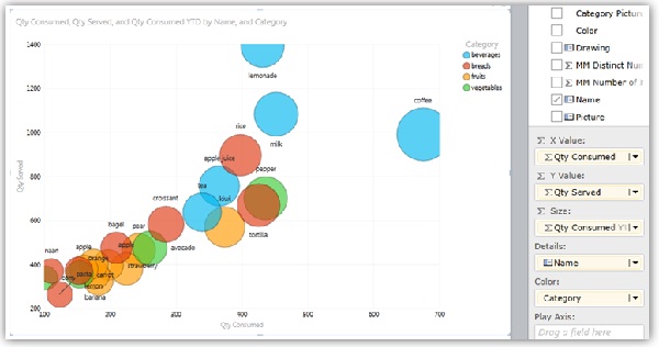
Bubble and scatter charts in Power View - Excel
Create a Pareto Chart in Excel (In Easy Steps) - Excel Easy If you don't have Excel 2016 or later, simply create a Pareto chart by combining a column chart and a line graph. This method works with all versions of Excel. 1. First, select a number in column B. 2. Next, sort your data in descending order. On the Data tab, in the Sort & Filter group, click ZA. 3. Calculate the cumulative count. Enter the ...
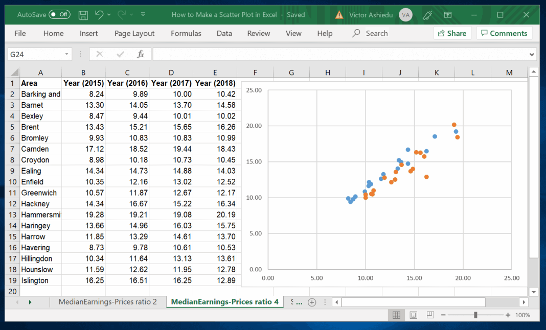
How to Make a Scatter Plot in Excel | Itechguides.com
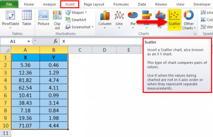
How To Create Scatter Chart in Excel? - EDUCBA To apply the scatter chart by using the above figure, follow the below-mentioned steps as follows. Step 1 – First, select the X and Y columns as shown below. Step 2 – Go to the Insert menu and select the Scatter Chart. Step 3 – Click on the down arrow so that we will get the list of scatter chart list which is shown below.
Add Custom Labels to x-y Scatter plot in Excel - DataScience Made Simple
Scatter Plots in Excel with Data Labels - LinkedIn Select "Chart Design" from the ribbon then "Add Chart Element" Then "Data Labels". We then need to Select again and choose "More Data Label Options" i.e. the last option in the menu. This will...
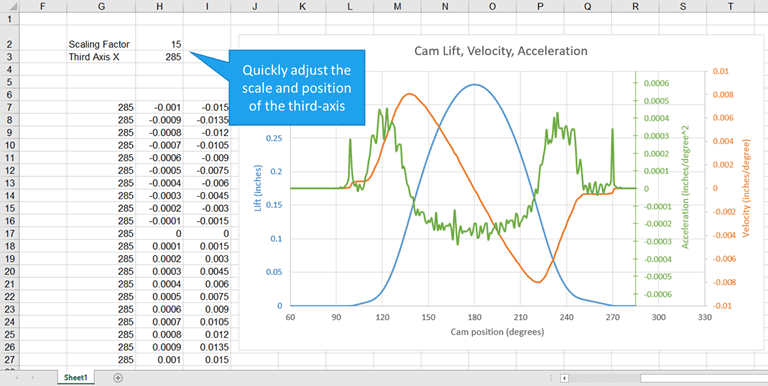
How to Add a Third Y-Axis to a Scatter Chart | EngineerExcel
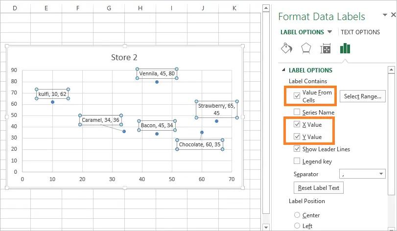
Add Custom Labels to x-y Scatter plot in Excel Step 1: Select the Data, INSERT -> Recommended Charts -> Scatter chart (3 rd chart will be scatter chart) Let the plotted scatter chart be. Step 2: Click the + symbol and add data labels by clicking it as shown below. Step 3: Now we need to add the flavor names to the label. Now right click on the label and click format data labels.

Module1
Dynamically Label Excel Chart Series Lines - My Online Training … 26.09.2017 · Hi Mynda – thanks for all your columns. You can use the Quick Layout function in Excel (Design tab of the chart) to do the labels to the right of the lines in the chart. Use Quick Layout 6. You may need to swap the columns and rows in your data for it to show. Then you simply modify the labels to show only the series name. I just happened to ...
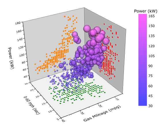
3D Graphs in Origin
mivp.teacherandstudent.de Click Correlation in the analysis window and click OK. 2. 3. Click on the Input Range box and highlight cells A1 to B13. Make sure you have the box next to Labels in first row clicked. 4. Click on the Output Range box and click cell B15. Click OK. The correlation coefficient will appear.
Post a Comment for "45 excel scatter chart data labels"