40 pivot table row labels format

changing Date format in a pivot table - Microsoft Tech Community Mar 04, 2019 · @Jan Karel PieterseI have a pivot table and chart in (current) Office 365 with dates in the row column; when I follow the same steps as described below, there is no "Number Format" button showing in the Field Settings dialog - see screen copy below.Why is that? I managed to change the date format within the pivot table (using "ungroup"), but this new … Conditional Formatting in Pivot Table - WallStreetMojo Currently, a pivot table is blank. Next, we need to bring in the values. Then, drag down the "Date" in the "Rows" Label, "Name" in the "Column," and "Sales" in "Values." As a result, the pivot table will look like the one below. To apply conditional formatting in the pivot table, first, we must select the column to format.

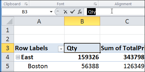
PDF Excel Troubleshooting Row Labels in Pivot Tables In Excel 2007 and earlier, you had to follow these steps: 1. Select the entire pivot table. 2. Copy the pivot table to the clipboard. 3. Use the Paste Special dialog to paste just the Values. This will change the report from a live pivot table to a static report. 4. Select the first blank column cell to the last blank column cell. 5.

Pivot table row labels format

How to Move Excel Pivot Table Labels Quick Tricks Jul 12, 2021 · Move Pivot Table Labels. This short video shows 3 ways to manually move the labels in a pivot table, and the written instructions are below the video. Drag a Label. Use Menu Commands. Type over a Label. Drag Labels to New Position. To move a pivot table label to a different position in the list, you can drag it: Click on the label that you want ... How to Format Pivot Tables in Google Sheets (Step by Step) Choose the "Pivot Table" option. Look for the field labeled "Insert to.". Choose if you want the pivot table on a "New Sheet" or "Existing Sheet.". Look for the section labeled "Data Range.". Enter the cells you want to include in the pivot table. You could type "A1:D1" without the quotation marks, for example. Excel Pivot Table Row labels - Stack Overflow 1 Answer. Right click on the pivot, go to PivotTable Options, Display Tab. Click on "Classic Pivot Table Layout". Go to each field (column), right click, field settings, layout & print tab. Click on "Repeat Item Labels". That should give you the table you're looking for.

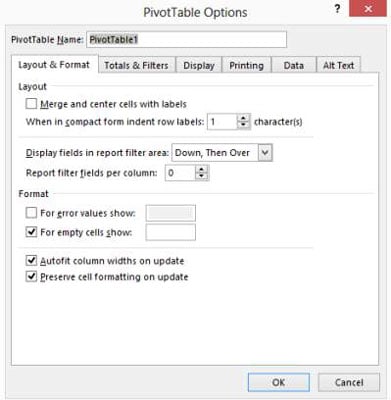
Pivot table row labels format. How to Format Excel Pivot Table - Contextures Excel Tips Jun 22, 2022 · Video: Change Pivot Table Labels. Watch this short video tutorial to see how to make these changes to the pivot table headings and labels. Get the Sample File. No Macros: To experiment with pivot table styles and formatting, download the sample file. The zipped file is in xlsx format, and and does NOT contain any macros. Design the layout and format of a PivotTable In the PivotTable Options dialog box, click the Layout & Format tab, and then under Layout, select or clear the Merge and center cells with labels check box. Note: You cannot use the Merge Cells check box under the Alignment tab in a PivotTable. Change the display of blank cells, blank lines, and errors How to make row labels on same line in pivot table? Make row labels on same line with PivotTable Options You can also go to the PivotTable Options dialog box to set an option to finish this operation. 1. Click any one cell in the pivot table, and right click to choose PivotTable Options, see screenshot: 2. Automate Pivot Table with Python (Create, Filter and Extract) May 22, 2021 · Automate Pivot Table and extract data from the filtered Pivot Table. Save your time for a cup of tea. Open in app. ... The input is the PS4 Games Sales in CSV format as shown in the image below. ... The “Values” and “Row Labels” are the Field Headers, not a Data Field. The script is the same as the action below.

Formatting Tips for Pivot Tables - Goodly Well the filter buttons are missing from the pivots. Here are 2 ways to get it. Method 1 : Is by choosing value filters in the filter drop down of the row labels. Method 2 : Selecting the adjacent cell outside the pivot and press CTRL SHIFT L. This will directly give you a filter on the Sales Values. Format Pivot Table Labels Based on Date Range In the pivot table, remove any filters that have been applied - all the rows need to be visible before you apply the conditional formatting. Select all the dates in the Row Labels that you want to format. On the Ribbon, click the Home tab, and then in the Styles group, click Conditional Formatting. How to Format the Values of Numbers in a Pivot Table Click the Insert tab, then Pivot Table. This will launch the Create PivotTable dialog box. Figure 3. Inserting a Pivot Table. Step 3. In the Create PivotTable dialog box, tick Existing Worksheet. Click the bar for Location and then click cell H2. This will position the pivot table in the existing worksheet, at cell H2. Figure 4. Pivot Table Formatting - Excel Champs Click anywhere on the PivotTable to activate the design tab. Now, click on the small drop-down arrow in the designs to scroll to the end. Here click on the "New PivotTable Style". Now, a pop-up window will open "New PivotTable Style". Rename the PivotTable in the "Name Field". Select an element to format and click on the "Format ...

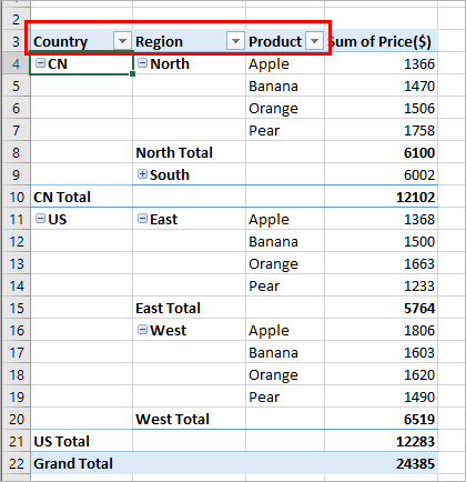
Pivot table row labels in separate columns • AuditExcel.co.za Our preference is rather that the pivot tables are shown in tabular form (all columns separated and next to each other). You can do this by changing the report format. So when you click in the Pivot Table and click on the DESIGN tab one of the options is the Report Layout. Click on this and change it to Tabular form. Conditional Formatting on Pivot Table row labels In srcFromPowerPivot sheet cell A is from powerpivot under row label comparing the dates in cell C (3 dates) and the condtional formatting doesnt work. In cell J it worked cos I dragged under value instead of row label. In the srcFromWorksheet it worked even though it is under rowlabel. Sheet3 is just a copy of powerpivot data. 101 Advanced Pivot Table Tips And Tricks You Need To Know Apr 25, 2022 · When using a pivot table your source data will need to be in a tabular format.This means your data is in a table with rows and columns. The first row should contain your column headings which describes the data directly below in that column. There should be no blank column headings in your data. How to Customize Your Excel Pivot Chart Data Labels - dummies To add data labels, just select the command that corresponds to the location you want. To remove the labels, select the None command. If you want to specify what Excel should use for the data label, choose the More Data Labels Options command from the Data Labels menu. Excel displays the Format Data Labels pane.

Repeat Pivot Table row labels • AuditExcel.co.za Pivot Tables Course

Formatting Row Labels in Pivot Table/Chart Any attempts to change the formatting of the row labels to 'h' is promptly ignored by Excel. Note the two tasks that occur at hour 18 (one at 18:00 and the other at 18:20 (you will need to see the formatting to truly see the minutes)). Those should be combined in the pivot table (and they are) and on my 'adjusted' table (where I used SUMIFS ...

Pivot Table in Excel - A Beginners Guide for Excel Users

Find the Source Data for Your Pivot Table – Excel Pivot Tables Feb 12, 2014 · Follow these steps, to find the source data for a pivot table: Select any cell in the pivot table. On the Ribbon, under the PivotTable Tools tab, click the Analyze tab (in Excel 2010, click the Options tab). In the Data group, click the top section of the Change Data Source command. In the Change PivotTable Data Source dialog box, you can see ...

Pivot Table Row Labels Side By Side | Decorations I Can Make

How to Create a Pivot Table in Excel: A Step-by-Step Tutorial Dec 31, 2021 · To automatically format the empty cells of your pivot table, right-click your table and click PivotTable Options. ... Drag and drop a field into the "Row Labels" area. Drag and drop a field into the "Values" area. Fine-tune your calculations. Now that you have a better sense of what pivot tables can be used for, let's get into the nitty-gritty ...

How to Set Pivot Table Options in Excel - dummies

Pivot Chart Data Label Formatting Question - Microsoft Tech Community Hi, I have a pivot chart. I format the data labels, for example make the text larger or turn it. Every time I refresh the data the data label formatting reverts to the default. I have gone to the Pivot Chart options and made sure the Preserve cell formatting option is checked. How to I get around...

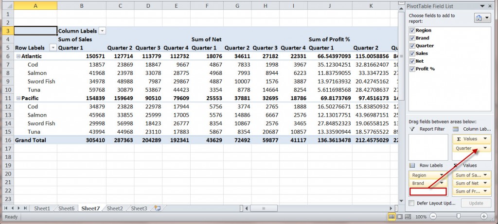
MS Excel 2013: Display the fields in the Values Section in a single column in a pivot table

Automatic Row And Column Pivot Table Labels - How To Excel At Excel Select the data set you want to use for your table The first thing to do is put your cursor somewhere in your data list Select the Insert Tab Hit Pivot Table icon Next select Pivot Table option Select a table or range option Select to put your Table on a New Worksheet or on the current one, for this tutorial select the first option Click Ok

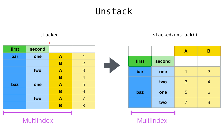
Reshaping and pivot tables — pandas 1.0.3 documentation

Excel pivot table conditional formatting row labels Jobs, Ansættelse ... Søg efter jobs der relaterer sig til Excel pivot table conditional formatting row labels, eller ansæt på verdens største freelance-markedsplads med 21m+ jobs. Det er gratis at tilmelde sig og byde på jobs.

Pivot table row labels in separate columns • AuditExcel.co.za

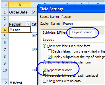
Repeat item labels in a PivotTable - support.microsoft.com Right-click the row or column label you want to repeat, and click Field Settings. Click the Layout & Print tab, and check the Repeat item labels box. Make sure Show item labels in tabular form is selected. Notes: When you edit any of the repeated labels, the changes you make are applied to all other cells with the same label.

Change Pivot Table Data Headings and Blanks – Excel Pivot Tables

How To Compare Multiple Lists of Names with a Pivot Table Jul 08, 2014 · 1. You can change the pivot table layout to Tabular format and Repeat the Labels. This is done from the Design tab in the ribbon with a cell in the pivot table selected. Here is a screenshot. 2. Another option is to concatenate/join the First Name and Last Name in a new column called Full Name. Then add this name to the pivot table.

Repeat Pivot Table row labels • AuditExcel.co.za Pivot Tables Course

How to Insert a Blank Row in Excel Pivot Table - MyExcelOnline Jan 17, 2021 · Pivot Table reports are shown in a Compact Layout format as a default and if you have two or more Items in the Row Labels (e.g.Month & Customer), then the Pivot Table report can look very clunky…. There is a cool little trick that most Excel users do not know about that adds a blank row after each item, making the Pivot Table report look more appealing.

How to Create a MS Excel 2010 Pivot Table – An Introduction | Technical Communication Center ...

Excel Pivot Table Row Label Column Display Format Now, I have a column whose datatype in database is integer, it is created as an hierarchy level, which can be brought as row, column or filter in Pivot Table. But the format in which it is showing is not right. Eg, It is showing like 200,911. instead i want to remove comma, and show row or column as . 200911

get a row label from pivot table - Microsoft Tech Community

Excel Pivot Table - Format Numbers in Rows To format rows or columns in a PT, hover the mouse at the top of the column or beginning of the row until a black arrow appears, click to highlight the row/column and format as usual. For Display labels from next field in same column, uncheck this, follow above procedure, then recheck. Paula Scharf

Get Rid of GetPivotData - Beat Excel!

Changing Blank Row Labels - Excel Pivot Tables You can manually change the (blank) labels in the Row or Column Labels areas by typing over them in the pivot table. You can type any text to replace the (Blank) entry, but you can't clear the cell and leave it empty: Select one of the Row or Column Labels that contains the text (blank). Type N/A in the cell, and then press the Enter key.

How to make row labels on same line in pivot table?

Overwrite pivot table conditional format based on row label As far as I know, using the one rule in the Conditional formatting, we can only format the cells with one color if the condition is true and if the same condition is false, the formatting of the cell will be blank and if both conditions are true, the formatting of cell depends on the highest ranking/priority of the rules in Conditional formatting.

Pivot table row labels side by side – Excel Tutorials

Pivot table row labels side by side - Excel Tutorials You can copy the following table and paste it into your worksheet as Match Destination Formatting. Now, let's create a pivot table ( Insert >> Tables >> Pivot Table) and check all the values in Pivot Table Fields. Fields should look like this. Right-click inside a pivot table and choose PivotTable Options…. Check data as shown on the image below.

Repeat Pivot Table Labels in Excel 2010 - Excel Pivot TablesExcel Pivot Tables

Change Pivot Table Layout using VBA - Access-Excel.Tips Even worse, the column label "Department" and "Empl ID" are gone. I personally hate this layout because it does not use the actual column name, instead it uses "Row Labels", "Column Labels". Since "Row Labels" refer to both Department and Empl ID as they display in one column, it uses a generic name "Row Labels".

33 Pivot Table Blank Row Label - Labels Database 2020

How to Create Excel Pivot Table (Includes practice file) Jun 28, 2022 · How to Create Excel Pivot Table. There are several ways to build a pivot table. Excel has logic that knows the field type and will try to place it in the correct row or column if you check the box. For example, numeric data such as Precinct counts tend to appear to the right in columns. Textual data, such as Party, would appear in rows. While ...

Share :